Optimal Control of a Rocket

This example is adapted from the JuMP tutorial.

The goal is to show that there are explicit repeated structures in discretized optimal control problem regarded as a nonlinear program (NLP). We will use the optimal control of a rocket as an example to demonstrate how to exploit these structures to solve the problem more efficiently via PyOptInterface.

Problem Formulation

The problem is to find the optimal control of a rocket to maximize the altitude at the final time while satisfying the dynamics of the rocket. The dynamics of the rocket are described by the following ordinary differential equations (ODEs):

\[\begin{split} \begin{align*} \frac{dh}{dt} &= v \\ \frac{dv}{dt} &= -g(h) + \frac{u-D(h,v)}{m} \\ \frac{dm}{dt} &= -\frac{u}{c} \end{align*} \end{split}\]

where \(h\) is the altitude, \(v\) is the velocity, \(m\) is the mass, \(u\) is the thrust, \(g(h)\) is the gravitational acceleration, and \(D(h,v)\) is the drag force. The thrust \(u\) is the control variable.

The drag force is given by \(D(h,v) = D_c v^2 \exp(-h_c \frac{h-h_0}{h_0})\), and the gravitational acceleration is given by \(g(h) = g_0 (\frac{h_0}{h})^2\).

By discretizing the ODEs, we obtain the following nonlinear program:

\[\begin{split} \begin{align*} \frac{h_{t+1}-h_t}{\Delta t} &= v_t \\ \frac{v_{t+1}-v_t}{\Delta t} &= -g(h_t) + \frac{u_t-D(h_t,v_t)}{m_t} \\ \frac{m_{t+1}-m_t}{\Delta t} &= -\frac{u_t}{c} \end{align*} \end{split}\]

where \(h_t\), \(v_t\), and \(m_t\) are the altitude, velocity, and mass at time \(t\), respectively, and \(\Delta t\) is the time step.

Implementation

In the discretized optimal control problem, the variables at two adjacent time points share the same algebraic relationship.

from math import sqrt
import pyoptinterface as poi
from pyoptinterface import nlfunc, ipopt

model = ipopt.Model()

h_0 = 1                      # Initial height
v_0 = 0                      # Initial velocity
m_0 = 1.0                    # Initial mass
m_T = 0.6                    # Final mass
g_0 = 1                      # Gravity at the surface
h_c = 500                    # Used for drag
c = 0.5 * sqrt(g_0 * h_0)    # Thrust-to-fuel mass
D_c = 0.5 * 620 * m_0 / g_0  # Drag scaling
u_t_max = 3.5 * g_0 * m_0    # Maximum thrust
T_max = 0.2                  # Number of seconds
T = 1_000                    # Number of time steps
delta_t = 0.2 / T;           # Time per discretized step

def rocket_dynamics(vars, params):
    m2, m1 = vars.m2, vars.m1
    h2, h1 = vars.h2, vars.h1
    v2, v1 = vars.v2, vars.v1
    u = vars.u

    h_eq = (h2 - h1) - delta_t * v1
    v_eq = (v2 - v1) - delta_t * (-g_0 * (h_0 / h1)**2 + (u - D_c * v1**2 * nlfunc.exp(-h_c * (h1 - h_0) / h_0)) / m1)
    m_eq = (m2 - m1) - delta_t * (-u / c)

    return [h_eq, v_eq, m_eq]

rd = model.register_function(rocket_dynamics)

---------------------------------------------------------------------------
ImportError                               Traceback (most recent call last)
Cell In[1], line 3
      1 from math import sqrt
      2 import pyoptinterface as poi
----> 3 from pyoptinterface import nlfunc, ipopt
      5 model = ipopt.Model()
      7 h_0 = 1                      # Initial height

ImportError: cannot import name 'nlfunc' from 'pyoptinterface' (/opt/hostedtoolcache/Python/3.12.10/x64/lib/python3.12/site-packages/pyoptinterface/__init__.py)

Then, we declare variables and set boundary conditions.

v = model.add_variables(range(T), name="v", lb=0.0, start=v_0)
h = model.add_variables(range(T), name="h", lb=0.0, start=h_0)
m = model.add_variables(range(T), name="m", lb=m_T, ub=m_0, start=m_0)
u = model.add_variables(range(T), name="u", lb=0.0, ub=u_t_max, start=0.0)

model.set_variable_bounds(v[0], v_0, v_0)
model.set_variable_bounds(h[0], h_0, h_0)
model.set_variable_bounds(m[0], m_0, m_0)
model.set_variable_bounds(u[T-1], 0.0, 0.0)

Next, we add the dynamics constraints.

for t in range(T-1):
    model.add_nl_constraint(
        rd,
        vars=nlfunc.Vars(h2=h[t+1], h1=h[t], v2=v[t+1], v1=v[t], m2=m[t+1], m1=m[t], u=u[t]),
        eq=0.0,
    )

Finally, we add the objective function. We want to maximize the altitude at the final time, so we set the objective function to be the negative of the altitude at the final time.

model.set_objective(-h[T-1])

After solving the problem, we can plot the results.

model.optimize()

h_value = []
for i in range(T):
    h_value.append(model.get_value(h[i]))

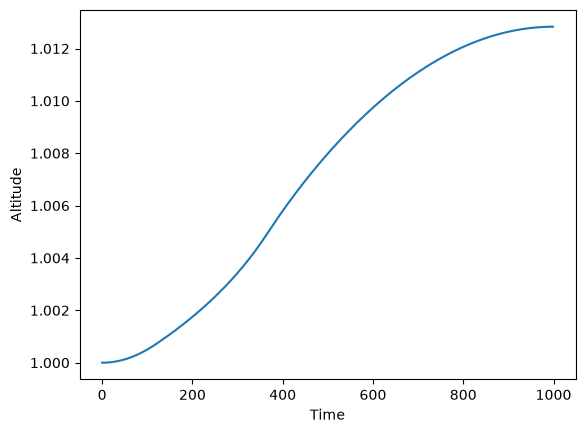
print("Optimal altitude: ", h_value[-1])

The plot of the altitude of the rocket is shown below.

import matplotlib.pyplot as plt

plt.plot(h_value)
plt.xlabel("Time")
plt.ylabel("Altitude")
plt.show()